Closed loop systems have the advantage of being self-contained and not dependent on external sources for calibration. After having verified the functionality of MASH modulation in achieving 1μV settability of the output voltage, correction of the DAC’s INL takes place through Newton’s method. The third-order polynomial coefficients are derived using an MCP3551 ADC, whose input range is limited to achieve sufficient linearity.
The key to achieving high resolution with a limited PWM counter wrap value is MASH modulation. I was first introduced to it through Andrew Holme’s website. The modulator generates a noise-shaped series of integer values, whose long-term average is the fractional input F divided by the counter modulo M. The values are then added to the PWM compare value to generate a high-resolution dithered PWM signal.
The code is directly adapted from Andrew’s website1 to work with the RP2040 C/C++ SDK.
// MASH state variables
static uint32_t q[4]    = {1, 0, 0, 0}; // Accumulators
static uint8_t  c[4][4] = {0};          // Carry flip-flops

// Computes the next value in the MASH sequence
int mash_next(uint32_t F)
{
    uint32_t d[4]; // Adder outputs

    // Carry flip-flop shift
    c[3][3] = c[3][2]; c[3][2] = c[3][1]; c[3][1] = c[3][0];
                       c[2][2] = c[2][1]; c[2][1] = c[2][0];
                                          c[1][1] = c[1][0];

    // Adders
    d[0] = (q[0] + F)    % modulo;
    d[1] = (q[1] + d[0]) % modulo;
    d[2] = (q[2] + d[1]) % modulo;
    d[3] = (q[3] + d[2]) % modulo;

    // Carries
    c[0][0] = (q[0] + F)    / modulo;
    c[1][0] = (q[1] + d[0]) / modulo;
    c[2][0] = (q[2] + d[1]) / modulo;
    c[3][0] = (q[3] + d[2]) / modulo;

    // Update latches
    memcpy(q, d, sizeof(q));

    // Compute output
    return c[0][0]
         + c[1][0] -     c[1][1]
         + c[2][0] - 2 * c[2][1] +     c[2][2]
         + c[3][0] - 3 * c[3][1] + 3 * c[3][2] - c[3][3];
}
I rewrote the code to be functionally and spectrally equivalent, while being better optimized to run on MCUs or FPGAs. According to Godbolt (ARM GCC 14.3.0 (unknown-eabi)), Andrew’s version is compiled to 200 lines of assembly, while mine compiles to 66 lines.
int MODULO = 16; // 16-bit equivalent accumulator
int FRAC = 1;

long integrator_1 = 0;
long integrator_2 = 0;
long integrator_3 = 0;
long integrator_4 = 0;
long feedback = 0;

int mash_next(uint32_t frac)
{
   integrator_1 += FRAC         - (feedback << MODULO);
   integrator_2 += integrator_1 - (feedback << MODULO);
   integrator_3 += integrator_2 - (feedback << MODULO);
   integrator_4 += integrator_3 - (feedback << MODULO);
   feedback = integrator_4 >> MODULO;
   return feedback;
}
The only disadvantage is that the modulo is necessarily a power of two, which makes the trick I used in the video difficult without involving division, which is a costly operation.
This is probably the part I found the most fascinating. I was initially unsure as to how the correction was supposed to be implemented. One idea was to calculate the INL error using a polynomial derived from Excel. The error value would then be divided by the DAC resolution to get the number of counts to be, depending on the sign, added to or subtracted from, the setpoint.
The polynomial transfer function’s inverse would ultimately be needed to calculate the corrected DAC setpoint for a given input. Rearranging a cubic equation of the form \(y = f(x)\) to \(x = g(y)\) didn’t seem like a particularly easy task that could be made to work for an arbitrary polynomial, so a modified version of Newton’s method was the only option.
#define TOLERANCE      1E-7  // 0.1 μV tolerance
#define MAX_ITERATIONS   10  // Max. Newton's method iterations

// Polynomial coefficients from Excel fit: LINEST(ys, xs^{1,2,3,4})
// const double A = +4.92829977769200E-28;  // x^4 coefficient
const double B = +5.99437550350965E-22;  // x^3 coefficient
const double C = -7.26799126246263E-13;  // x^2 coefficient
const double D = +1.00005657765389E+00;  // x^1 coefficient
const double E = -4.02676162926114E+02;  // x^0 coefficient

// 3rd order correction
int32_t correct_dac_input(int32_t v_target)
{
    double x = (double)v_target; // Start with the target value

    for (int i = 0; i < MAX_ITERATIONS; i++)
    {
        double x2 = x * x;  // x²
        double x3 = x2 * x; // x³

        // Compute f(x) = B*x³ + C*x² + D*x + E - v_target
        double f_x = (B * x3) + (C * x2) + (D * x) + E - v_target;

        // Compute f'(x) = 3B*x² + 2C*x + D
        double f_prime_x = (3.0 * B * x2) + (2.0 * C * x) + D;

        // Stop if within tolerance or derivative is too small
        if (fabs(f_x) < TOLERANCE || fabs(f_prime_x) < 1e-12)
        {
            break;
        }

        // Newton's update step: x_new = x - (f(x) / f'(x))
        x -= f_x / f_prime_x;
    }

    return (int32_t)round(x); // Convert final result to integer μV
}
Everything apart from double f_x = (B * x3) + (C * x2) + (D * x) + E - v_target; is a conventional implementation of Newton’s Method. What makes the calculation of a local inverse possible is - v_target, which subtracts the input setpoint from the transfer function, making the corrected setpoint the ‘zero’ of this new function, which the algorithm calculates within a couple of cycles.
It is interesting to take a look at the variable values at each iteration of the function with different inputs.
The coefficients used:
const double B = -8.28430452439943E-21;  // x^3 coefficient
const double C = +8.73115809293427E-12;  // x^2 coefficient
const double D = +1.00001955300857E+00;  // x^1 coefficient
const double E = -1.31753654978901E+03;  // x^0 coefficient
Input -1000000:
F:  -1328.3501160, F':     +1.0000021, X: -1000000.000000
F:     +0.0000154, F':     +1.0000021, X: -998671.6526282
F:     -0.0000000, F':     +1.0000021, X: -998671.6526436
Final X: -998671.6526436
Corrected input: -998672
Input 0:
F:  -1317.5365498, F':     +1.0000196, X:     +0.0000000
F:     +0.0000152, F':     +1.0000196, X:  +1317.5107885
F:     +0.0000000, F':     +1.0000196, X:  +1317.5107733
Final X:   1317.5107733
Corrected input: 1318
Now, with an input of 1000000:
F:  -1289.2606674, F':     +1.0000370, X: +1000000.0000000
F:     +0.0000145, F':     +1.0000370, X: +1001289.2129788
F:     +0.0000000, F':     +1.0000370, X: +1001289.2129644
Final X: 1001289.2129644
Corrected input: 1001289
The first derivative of the function does not change (to 1E-07) in the small correction range. In this case, a simple linear approximation by adding the value of the polynomial function at the desired setpoint to it would suffice, but Newton’s method provides more flexibility for a large range of polynomial coefficients. Convergence is also relatively quick; the tolerance is reached in three iterations.
Closing the loop completely would require breaking my reliance on Excel to calculate the polynomial coefficients using LINEST(Y, X^{1,2,3}). It was rather challenging to find something suitable to adapt on the internet. The good old ‘Numerical Recipes’2 only had something called a Savitzky-Golay filter, and the code (and the mathematics behind it) went right over my head, not to mention the required libraries that I’d have to deal with. I desired a simple, no-strings-attached standalone implementation for the RP2040. I lucked out and found an obscure (and admittedly strange) website3. Although there was talk of Gauss-Jordan elimination (which is fresh in my head from last semester) and pivoting, a generic adaptation worked to fulfil my needs.
// Computes polynomial coefficients from pairs of x and y values
void polynomial_least_squares(int n, int order, double x[], double y[], double b[])
{
    double sum[2 * order + 1];
    double a[order + 1][order + 2];

    // Initialize sum array
    for (int i = 0; i < 2 * order + 1; i++)
    {
        sum[i] = 0;
    }

    // Compute sums
    for (int i = 0; i < n; i++)
    {
        double x_pow = 1;
        for (int j = 0; j < 2 * order + 1; j++)
        {
            sum[j] += x_pow;
            x_pow *= x[i];
        }
    }

    // Construct augmented matrix
    for (int i = 0; i <= order; i++)
    {
        for (int j = 0; j <= order; j++)
        {
            a[i][j] = sum[i + j];
        }
        a[i][order + 1] = 0;
        for (int j = 0; j < n; j++)
        {
            a[i][order + 1] += pow(x[j], i) * y[j];
        }
    }

    // Gaussian elimination with row swapping
    for (int k = 0; k <= order; k++)
    {
        int max_row = k;
        for (int i = k + 1; i <= order; i++)
        {
            if (fabs(a[i][k]) > fabs(a[max_row][k]))
            {
                max_row = i;
            }
        }
        if (max_row != k)
        {
            for (int j = 0; j <= order + 1; j++)
            {
                double temp = a[k][j];
                a[k][j] = a[max_row][j];
                a[max_row][j] = temp;
            }
        }
        for (int i = k + 1; i <= order; i++)
        {
            double factor = a[i][k] / a[k][k];
            for (int j = k; j <= order + 1; j++)
            {
                a[i][j] -= factor * a[k][j];
            }
        }
    }

    // Back-substitution
    for (int i = order; i >= 0; i--)
    {
        b[i] = a[i][order + 1];
        for (int j = i + 1; j <= order; j++)
        {
            b[i] -= a[i][j] * b[j];
        }
        b[i] /= a[i][i];
    }
}
The inputs to the function are fairly self-explanatory: An \(n^{th}\) order polynomial is to be fitted to arrays of x and y values of size n, and the \(n + 1\) generated coefficients stored in b. Basic mathematical limitations still apply - fitting an \(n^{th}\) order polynomial requires at least \(n + 1\) pairs of \(x\) and \(y\) values. More pairs results in a better fit for a given \(n\).
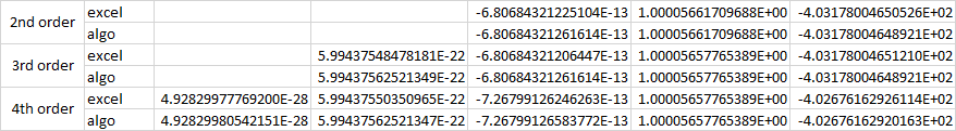
Comparing the values generated by the above function to Excel’s LINEST(), there are small differences, which I attribute to Excel performing additional statistics (which I don’t fully understand) on the values.
Although I was ultimately unable to close the loop due to various complications mentioned in the video, the basic C/C++ code for Newton’s method and polynomial LLS will certainly come in handy in the future - if not only for myself. The above code has also been empirically tested to be working.